Workflow Tutorial

This tutorial walks through a complete enzyme redesign session using CYP450 (PDB ID: 1SUO) as the case study. You will learn how to identify design hotspots, generate virtual saturation mutagenesis libraries, rationally evaluate mutants, cluster candidates, cross-screen with external tools, and explore co-evolution constraints.

Prerequisites

• REvoDesign installed and working in PyMOL
• Evolution data (PSSM + GREMLIN) pre-computed for your target sequence (see below)

Obtaining Evolution Data

REvoDesign requires PSSM and GREMLIN profiles computed from sequence databases. Use the computation service:

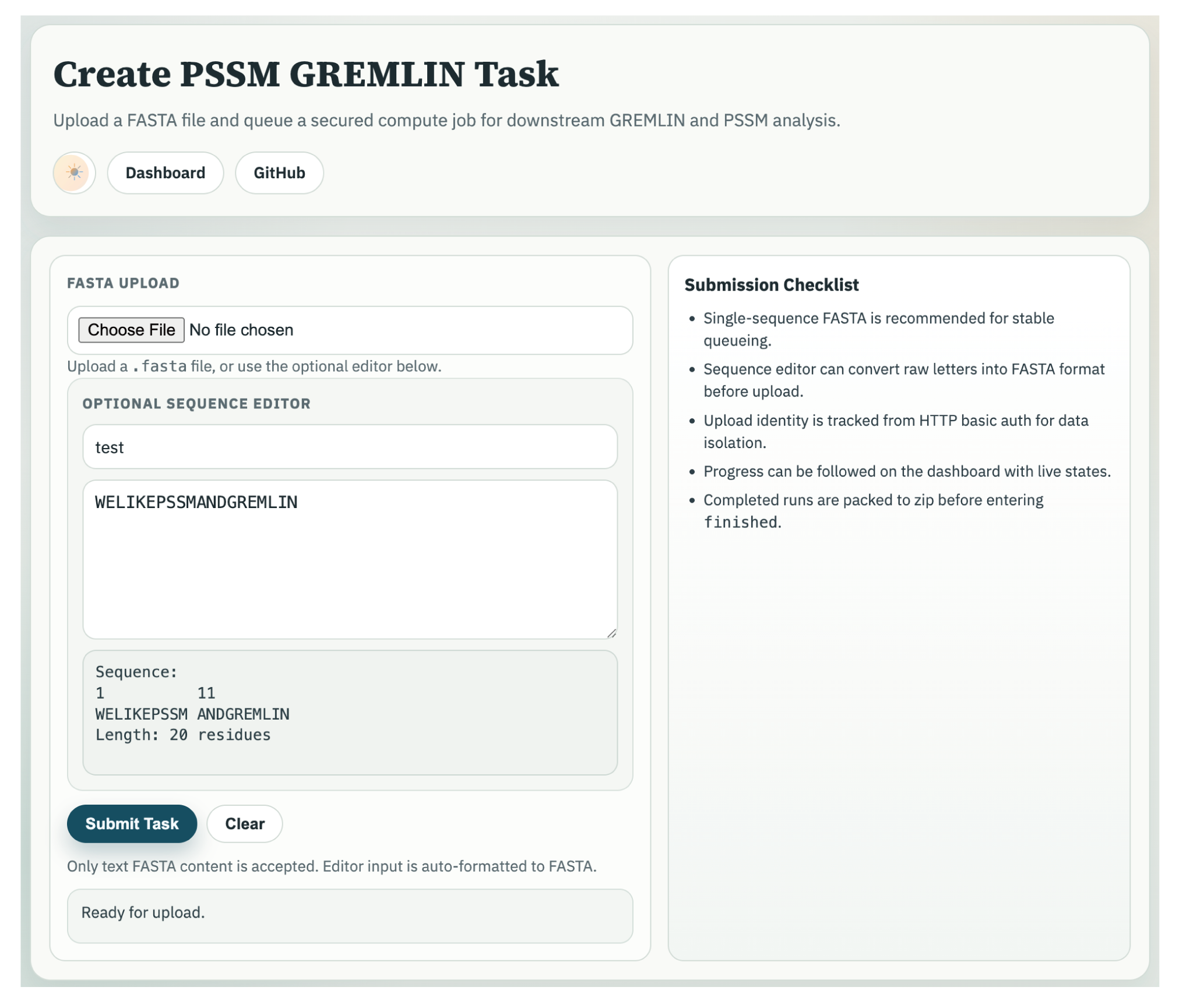
1. Go to https://revodesign.yaoyy.moe/PSSM_GREMLIN/create_task
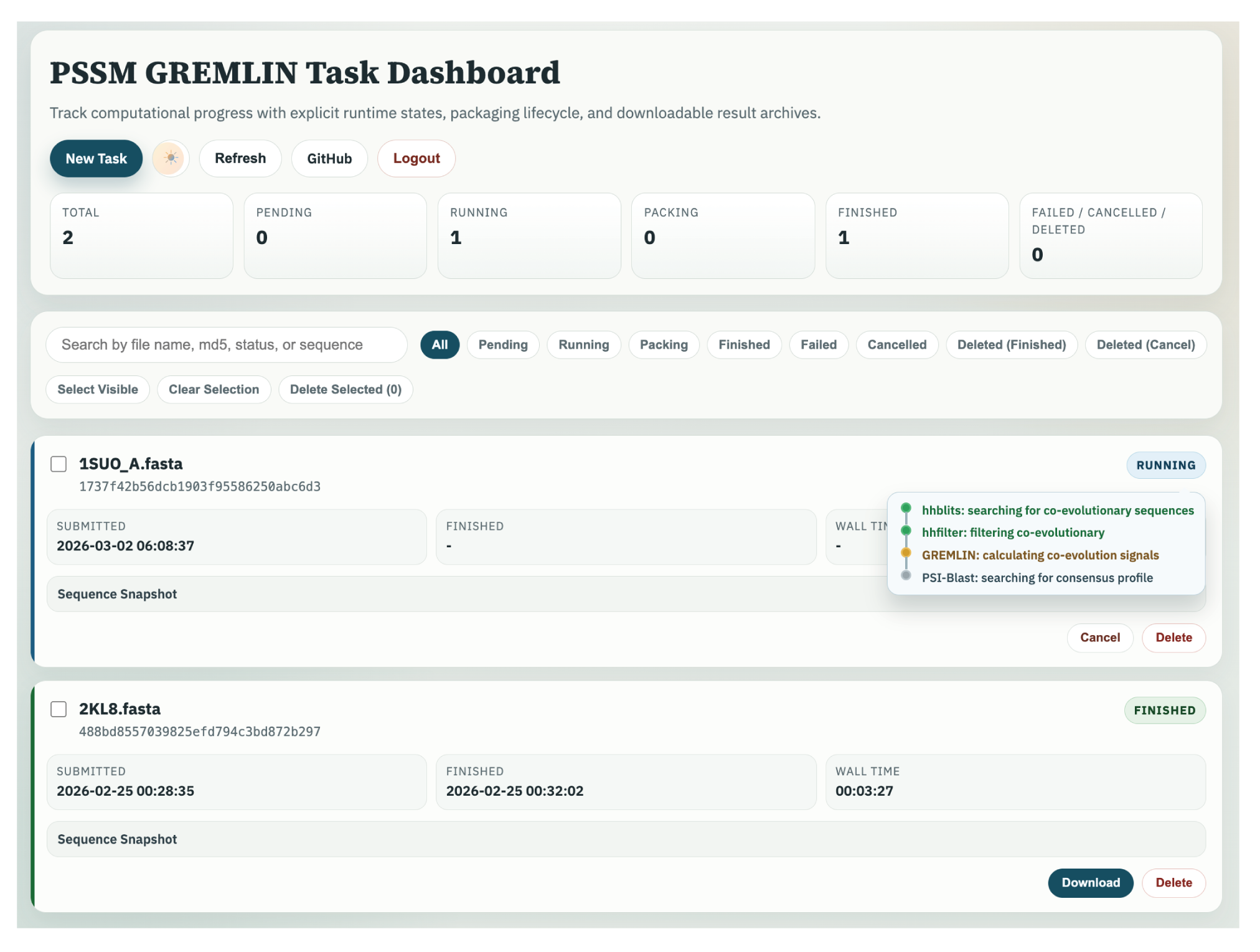
2. Upload a FASTA-format sequence file (one sequence per file). Sequences may contain unknown residues (X) but not stop codons (*).
3. Monitor progress at the Dashboard.
4. Hover over a task to reveal a cancel button (if queued/running) or a download button (if complete).
5. When complete, download and unzip the archive for use in the Prepare step.

PSSM/GREMLIN server task submission: upload a single FASTA file or paste a sequence

PSSM/GREMLIN server dashboard: monitor task status, cancel queued/running jobs, download completed results

Example FASTA

>1SUO_A
XXXXXXXXXXXXXXXXXXXXXXXXXXXGKLPPGPSPLPVLGNLLQMDRKGLLRSFLRLREKYGDVFTVYLGSRPVVVLCGTDAIREALVDQAEAFSGRGKIAVVDPIFQGYGVIFANGERWRALRRFSLATMRDFGMGKRSVEERIQEEARCLVEELRKSKGALLDNTLLFHSITSNIICSIVFGKRFDYKDPVFLRLLDLFFQSFSLISSFSSQVFELFSGFLKYFPGTHRQIYRNLQEINTFIGQSVEKHRATLDPSNPRDFIDVYLLRMEKDKSDPSSEFHHQNLILTVLSLFFAGTETTSTTLRYGFLLMLKYPHVTERVQKEIEQVIGSHRPPALDDRAKMPYTDAVIHEIQRLGDLIPFGVPHTVTKDTQFRGYVIPKNTEVFPVLSSALHDPRYFETPNTFNPGHFLDANGALKRNEGFMPFSLGKRICLGEGIARTELFLFFTTILQNFSIASPVPPEDIDLTPRESGVGNVPPSYQIRFLARH

Step 1: Prepare the Structure

Load and Set Up in PyMOL

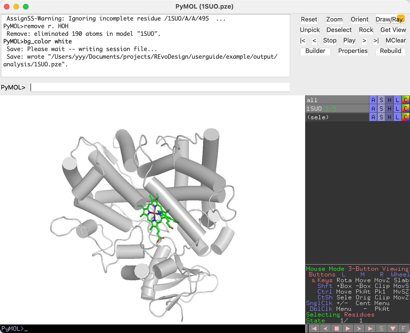
In PyMOL, fetch the target structure and prepare it for analysis:

fetch 1SUO

1SUO is a CYP450 enzyme with four components:

Segment ID	Molecule	Description
A	Protein	Enzyme
B	HEM	Cofactor
C	CPZ	Substrate
D	HOH	Crystallization water

Apply basic styling and clean up:

# Cartoon styling
set cartoon_cylindrical_helices, 1
set cartoon_color, gray70
set cartoon_transparency, 0.3

# Fix secondary structure assignment
dss

# Remove crystallization water
remove resn HOH

# White background
bg_color white

Save this session — it will serve as the starting point for all subsequent analysis.

Prepared 1SUO structure with cartoon styling

Import Session into REvoDesign

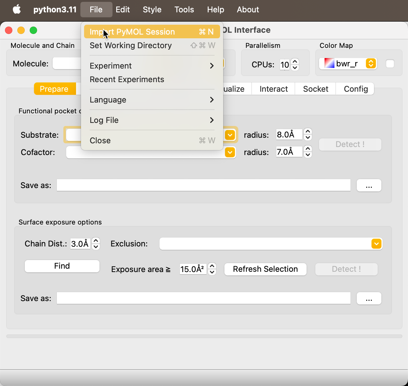
In REvoDesign, go to File → Import PyMOL Session (or press Ctrl+N / Cmd+N). This registers the PyMOL session so REvoDesign can identify molecules and selections.

Import the current PyMOL session into REvoDesign

Detect Binding Pocket Hotspots

In the Prepare tab, under the Pocket section:

1. Identify the substrate and cofactor molecules by their residue names (e.g., CPZ for the substrate, HEM for the cofactor).
2. Set the contact distance cutoff for each (default: 8 Å for substrate, 7 Å for cofactor).
3. Specify a save path to enable the detection button.
4. Click Detect.

Specify the substrate (CPZ) and cofactor (HEM) molecules

Set contact distances and save path, then click Detect

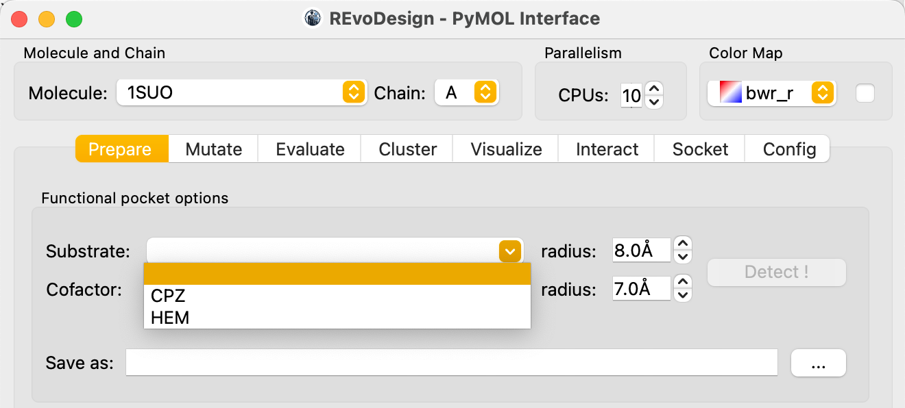
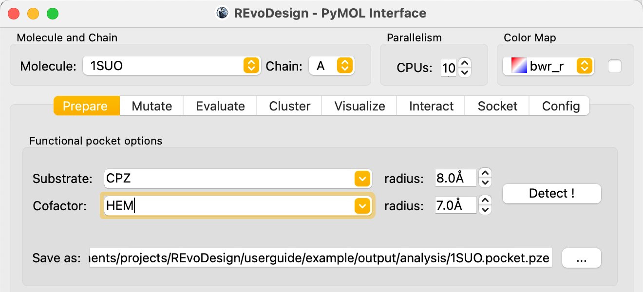
You can also use PyMOL selection syntax for complex cases (e.g., r. UNK or r. LIG to treat two ligands as one).

How pocket detection works

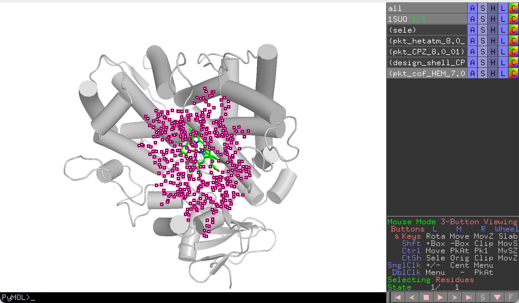
Residues within the cutoff distance of the substrate/cofactor are collected into selection groups. Overlapping regions (shared by cofactor and substrate) are assigned to the cofactor group and removed from the substrate group to avoid double-counting.

Results are saved to pockets/ in the working directory as <molecule>_<pocket_selection>_residues.txt. The following selections are created:

Selection	Content
design_shell_CPZ_8.0_01	Substrate-binding residues (cofactor overlap removed)
pkt_cof_HEM_7.0_01	Cofactor-binding residues
pkt_CPZ_8.0_01	Substrate-binding residues (full)
pkt_hetatm_8.0_01	All heteroatom-contacting residues (union)

Pocket detection results loaded into PyMOL

Detect Surface-Exposed Hotspots

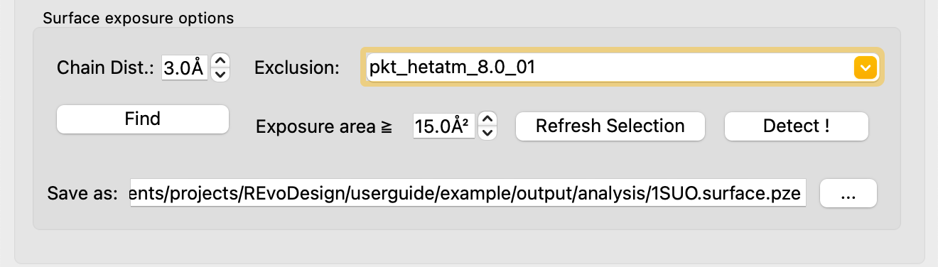
In the Prepare tab, under the Surface Exposure section:

1. Set the solvent-accessible surface area (SASA) threshold (default: 15 Ų). Residues with SASA ≥ threshold are considered surface-exposed.
2. Optionally exclude pocket residues: click Refresh Selection to load available PyMOL selections, then choose pkt_hetatm_8.0_01 from the Exclusion dropdown.
3. Specify a save path and click Find.

Surface exposure and PPI interface detection options

Set exclusion, SASA threshold, and save path

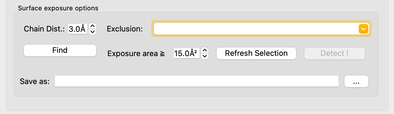
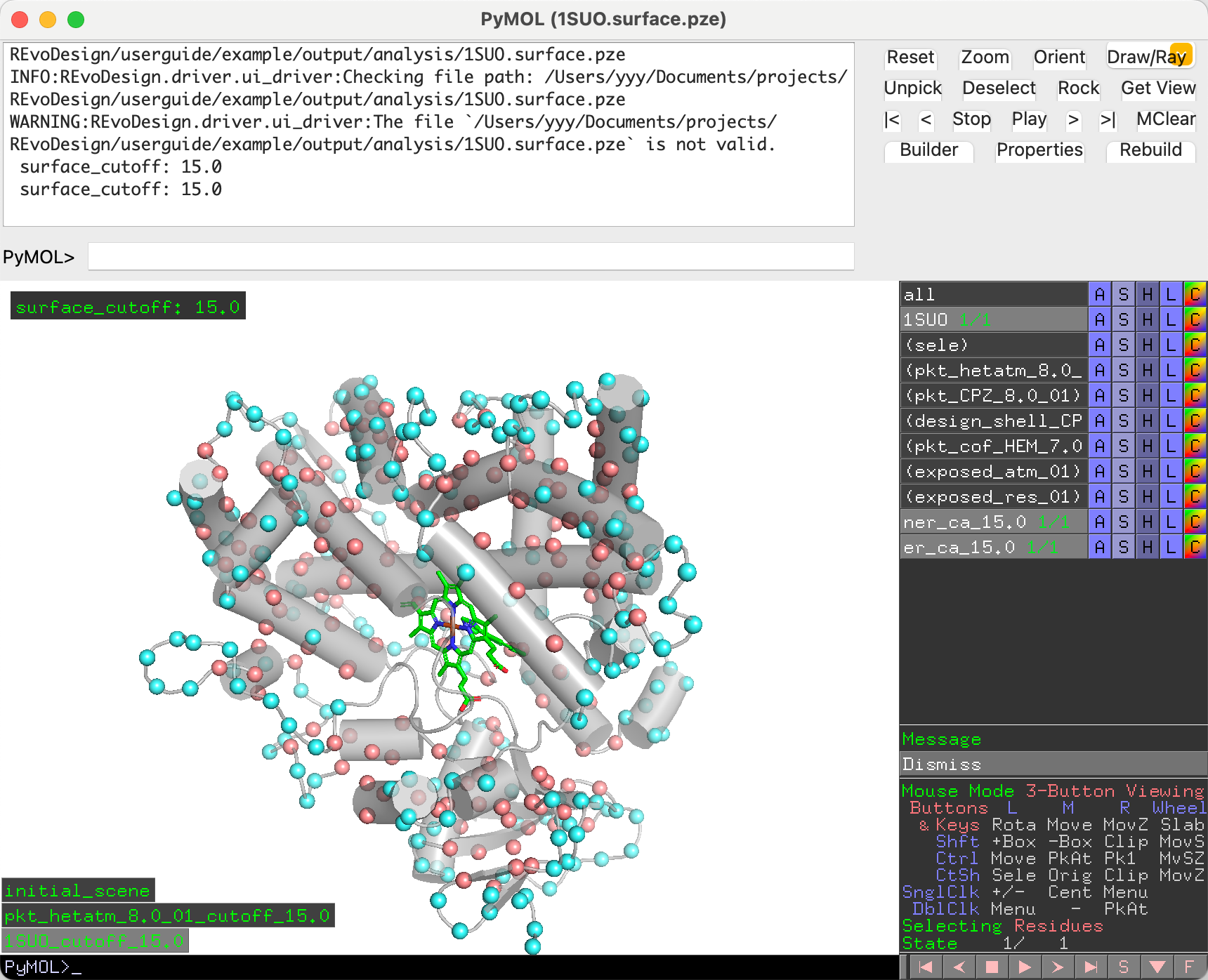
Results are visualized as spheres: blue for exposed, red for buried, and no sphere for excluded residues. Results are also saved to surface_residue_records/ in the working directory.

Surface exposure detection results (blue = exposed, red = buried)

Warning

The surface-exposure visualization session is for inspection only. Do not use it as the basis for further design steps — use the pre-detection session instead.

Protein-Protein Interface (Optional)

For multimeric proteins, use the PPI section to detect chain-chain contacts:

1. Set Chain Dist to the minimum contact distance between chains.
2. Click Find to identify interfacial residues.
3. Click Refresh Selection to load the result for exclusion.

Step 2: Mutate — Virtual Saturation Mutagenesis

The Mutate tab generates a pool of virtual point mutations under constraints derived from evolutionary conservation (PSSM).

Strategy 1: Surface Entropy Reduction

Surface entropy reduction replaces exposed residues with shorter, less solvent-interacting amino acids within conservation constraints.

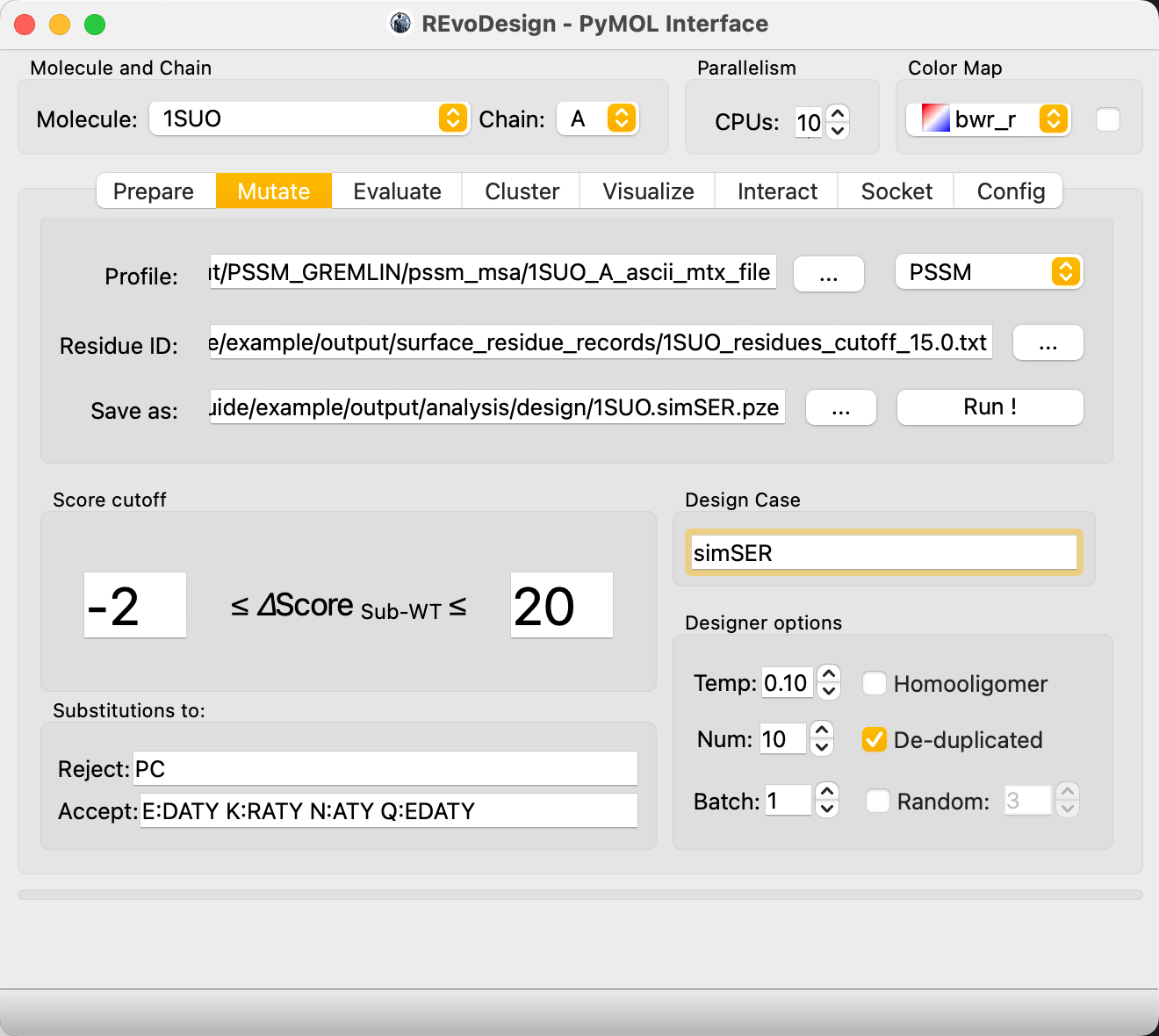
1. Load the unzipped evolution data into Profile and set type to PSSM.
2. Set Residue ID to the surface exposure result selection.
3. Choose a session save path.
4. Set Score cutoff bounds. Example: PSSM score difference ≥ -2 and ≤ 20 relative to wild-type (-2 tolerates slightly less conserved substitutions; 20 is effectively unbounded, meaning absolute conservation).
5. In Substitution:
   • Reject: PC (reject proline and cysteine)
   • Accept: e.g., E:DATY (replace E with D/A/T/Y candidates)
6. Enter a Design Case name for output file naming.
7. Click Run!

Surface entropy reduction design settings

Strategy 2: Catalytic Pocket Design

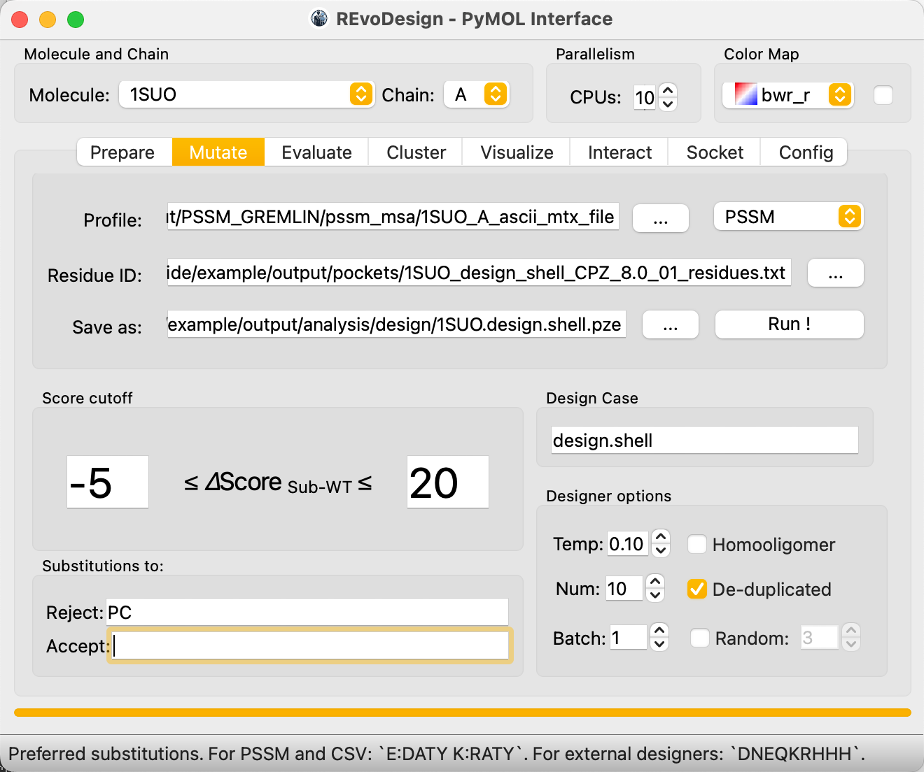
Catalytic pocket design uses a more permissive substitution strategy to increase diversity near the active site.

1. Set Score cutoff to a wider range (e.g., ≥ -5, ≤ 20).
2. Clear the Accept substitution preferences to allow all valid substitutions.
3. Keep Reject as PC to avoid disruptive proline/cysteine mutations.

Catalytic pocket design with relaxed conservation constraints

Understanding the Output

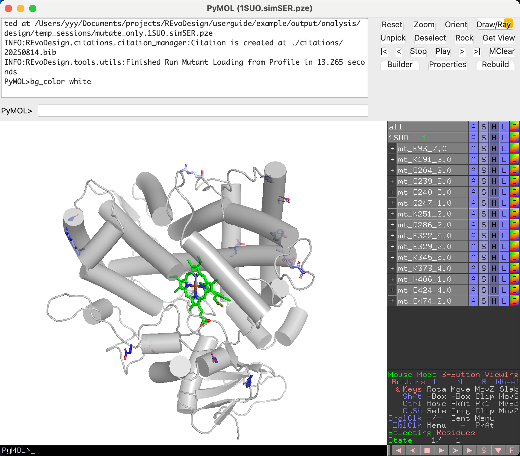
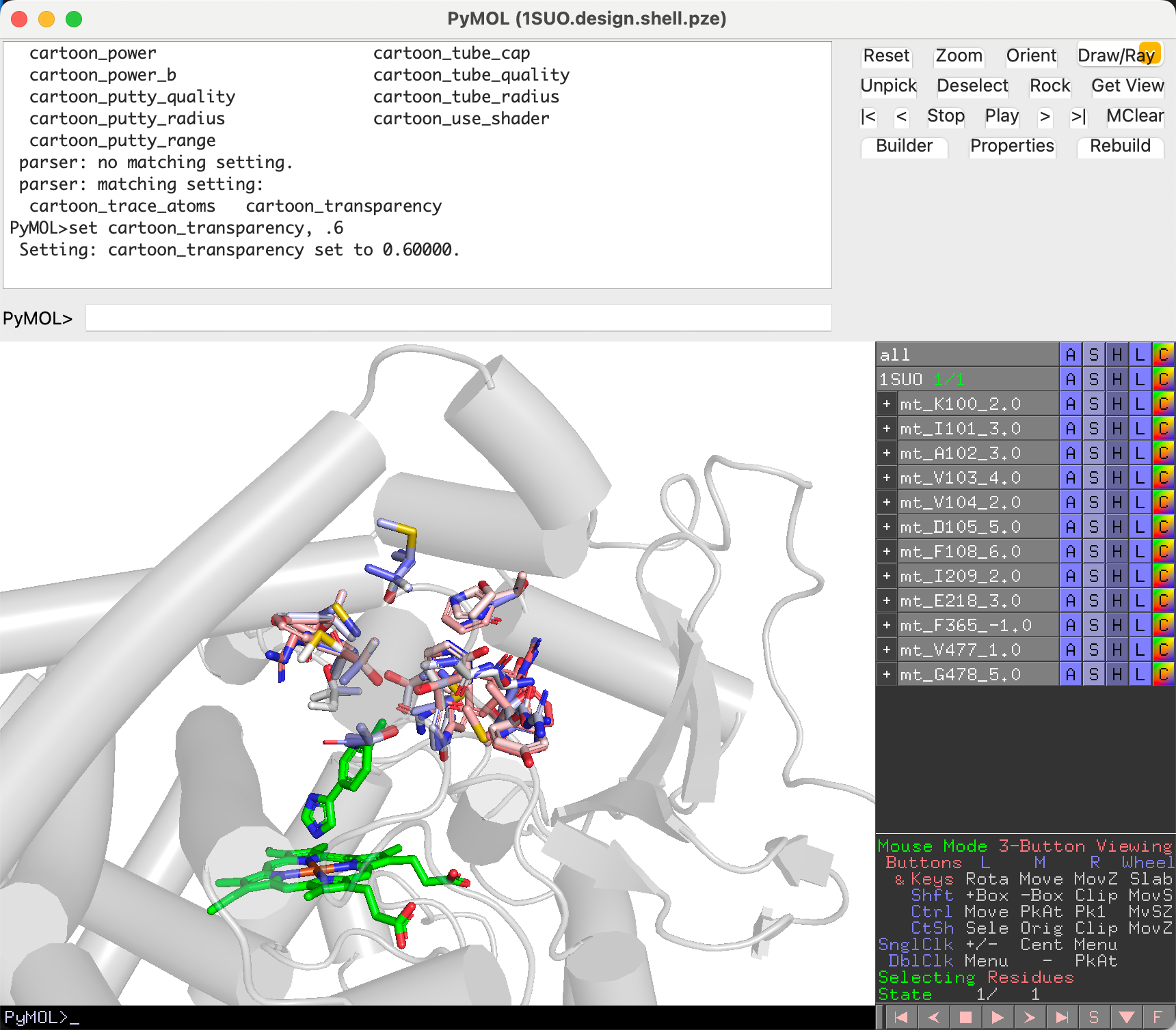
Design results appear in PyMOL grouped by residue position:

• Group name: mt_<WT><position>_<PSSM_score>
• Mutant name: <chain><WT><position><mutant>_<mutant_score>
• Only the mutated sidechain is shown
• Carbon atoms are colored by PSSM score (see color preset)
• Full PDB structures are saved under mutant_pdbs/ in the working directory

Surface entropy reduction — each group is a position, each entry a point mutant

Catalytic pocket design results

Step 3: Evaluate — Rational Screening

The Evaluate tab provides tools for visual, side-by-side comparison of wild-type and mutant sidechains to make informed decisions.

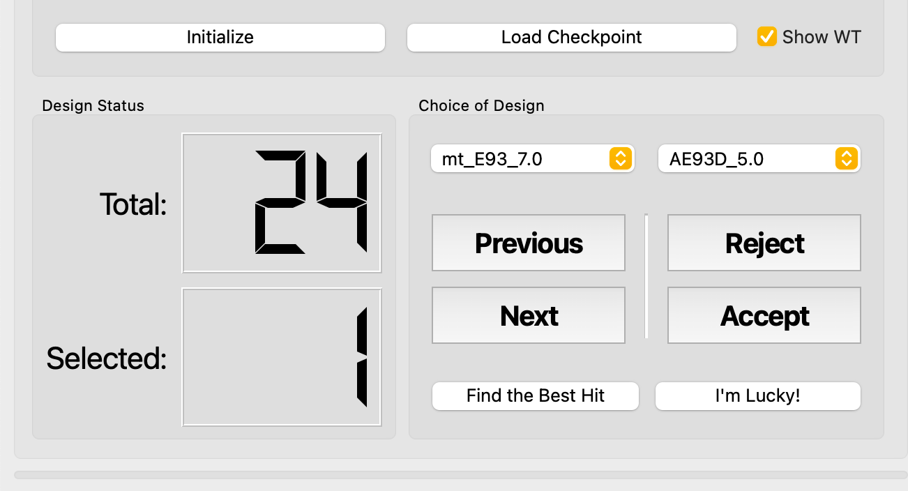
Initialize the MutantTree

REvoDesign organizes mutants into a MutantTree — branches are residue positions, leaves are individual point mutants at that position.

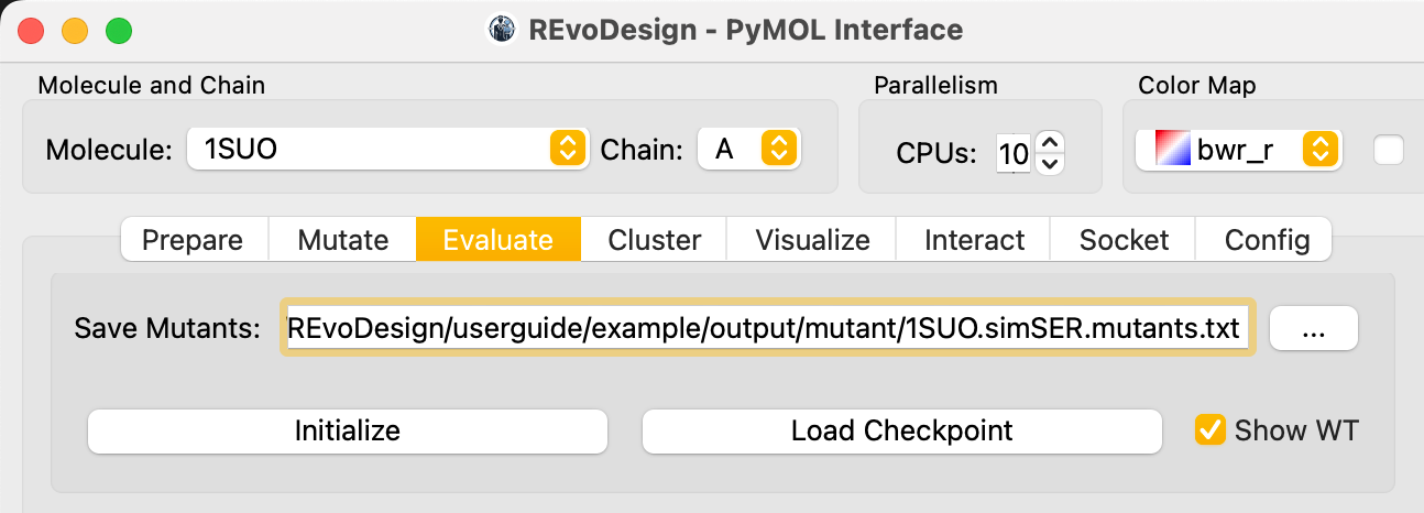
1. Go to the Evaluate tab.
2. Set a save path for mutant records and checkpoint files.
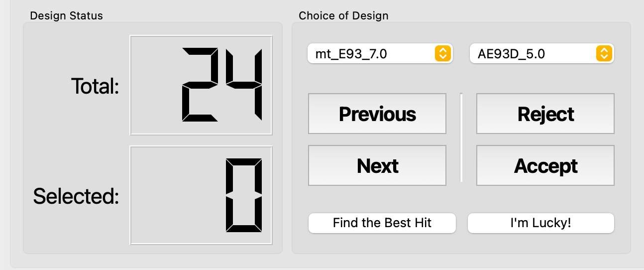
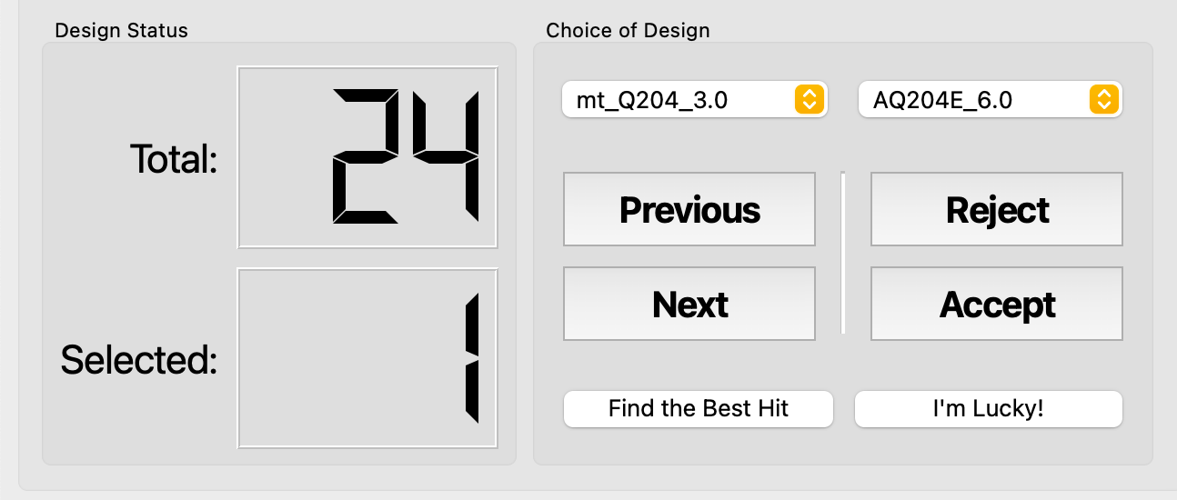
3. Click Initialize to scan the PyMOL session for mutant trees. If successful, Total shows a non-zero count and decision buttons become enabled.

Set save path for decision records and checkpoint files

Evaluation status: total mutants, accepted count, navigation and decision tools

Navigate and Decide

In evaluation mode, REvoDesign hides all other mutants, collapses unrelated branches, and shows only the current branch and individual. The wild-type sidechain is displayed as a wireframe for comparison, while the mutant sidechain is shown in ball-and-stick with a mesh surface.

Evaluation mode — wild-type (wireframe) vs mutant (ball-and-stick + mesh)

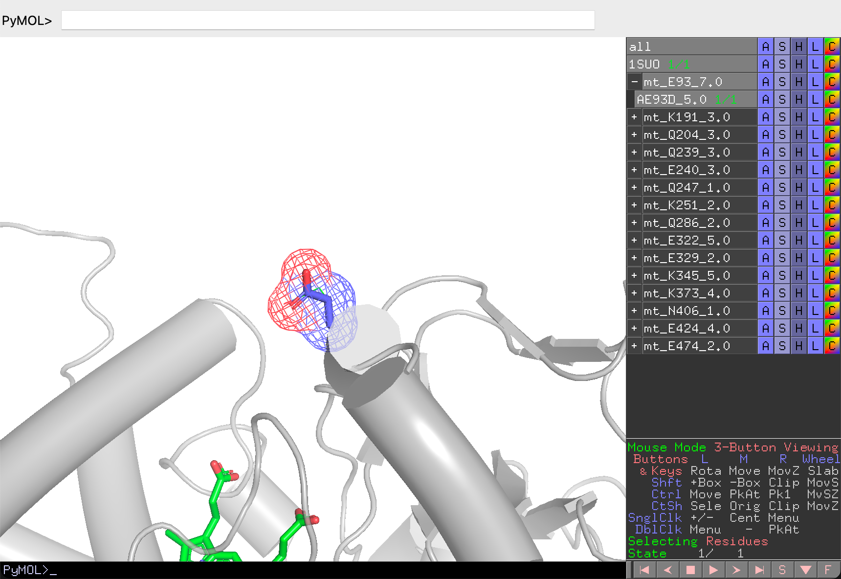
Decision actions:

Button	Action	Description
Previous	Go to previous mutant	Tooltip: Shift+Opt+[
Next	Go to next mutant	Tooltip: Shift+Opt+]
Accept	Accept current mutant	Tooltip: Shift+Opt+-
Reject	Reject current mutant	Tooltip: Shift+Opt++

Review and select the best-scoring mutant in a branch

After accepting, the decision state updates immediately

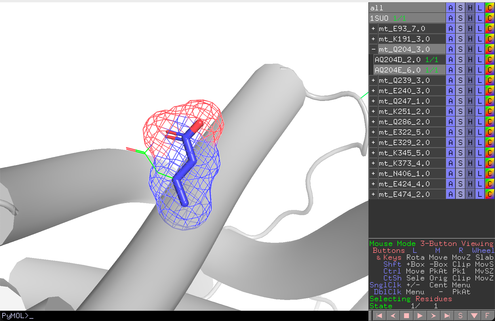
Fast Navigation

Use the dropdown menus to jump directly to a specific branch or mutant.

Jump to any branch via the dropdown

Select a specific point mutant within a branch

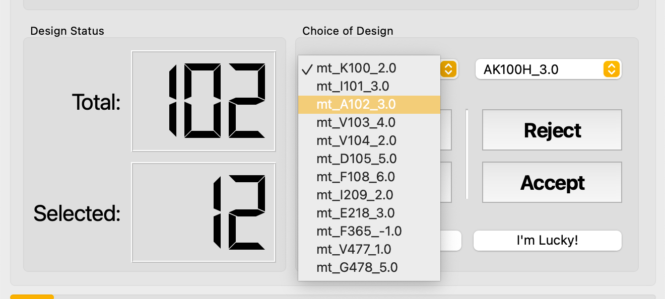
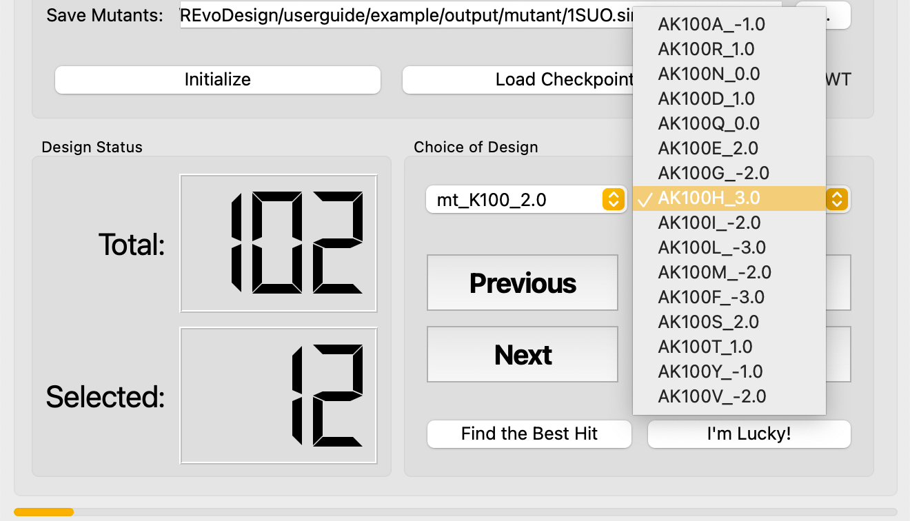
• Find the Best Hit — automatically jumps to the highest-scoring mutant in the current branch.

Click "Find the Best Hit" to jump to the branch's top scorer

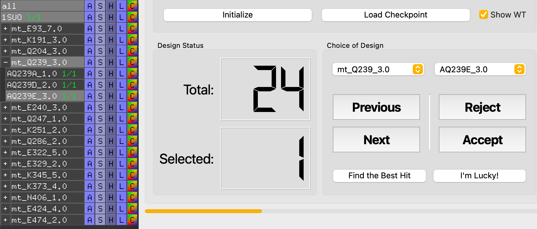
• I'm Lucky! — scans every branch and collects the highest-scoring mutant from each. This is a rapid way to identify promising leads across all positions.

"I'm Lucky!" automatically collects the best mutant from each branch

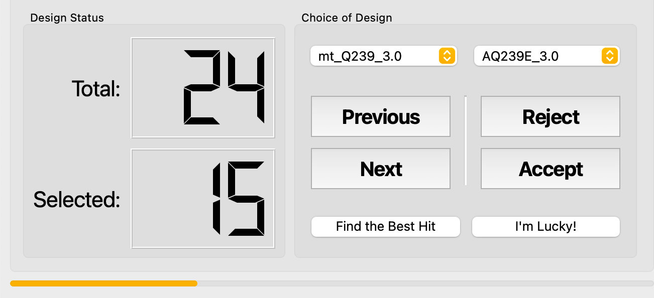
Decision Persistence

Decision results are saved in real time to a text file, with corresponding checkpoint files for reloading.

Real-time decision records saved to a text file

Checkpoint files allow resuming evaluation sessions

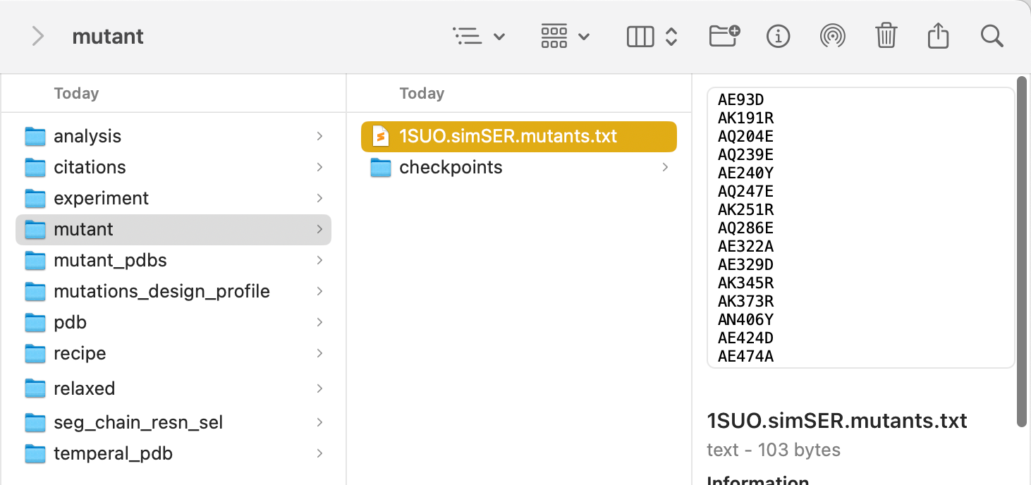
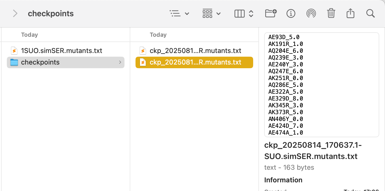
To reload a previous checkpoint:

1. Re-initialize the MutantTree (clears previous decisions).
2. Load the checkpoint file.
3. Previous decisions are restored.

Checkpoint loaded — previous decisions restored

Step 4: Cluster — Reduce Library Size

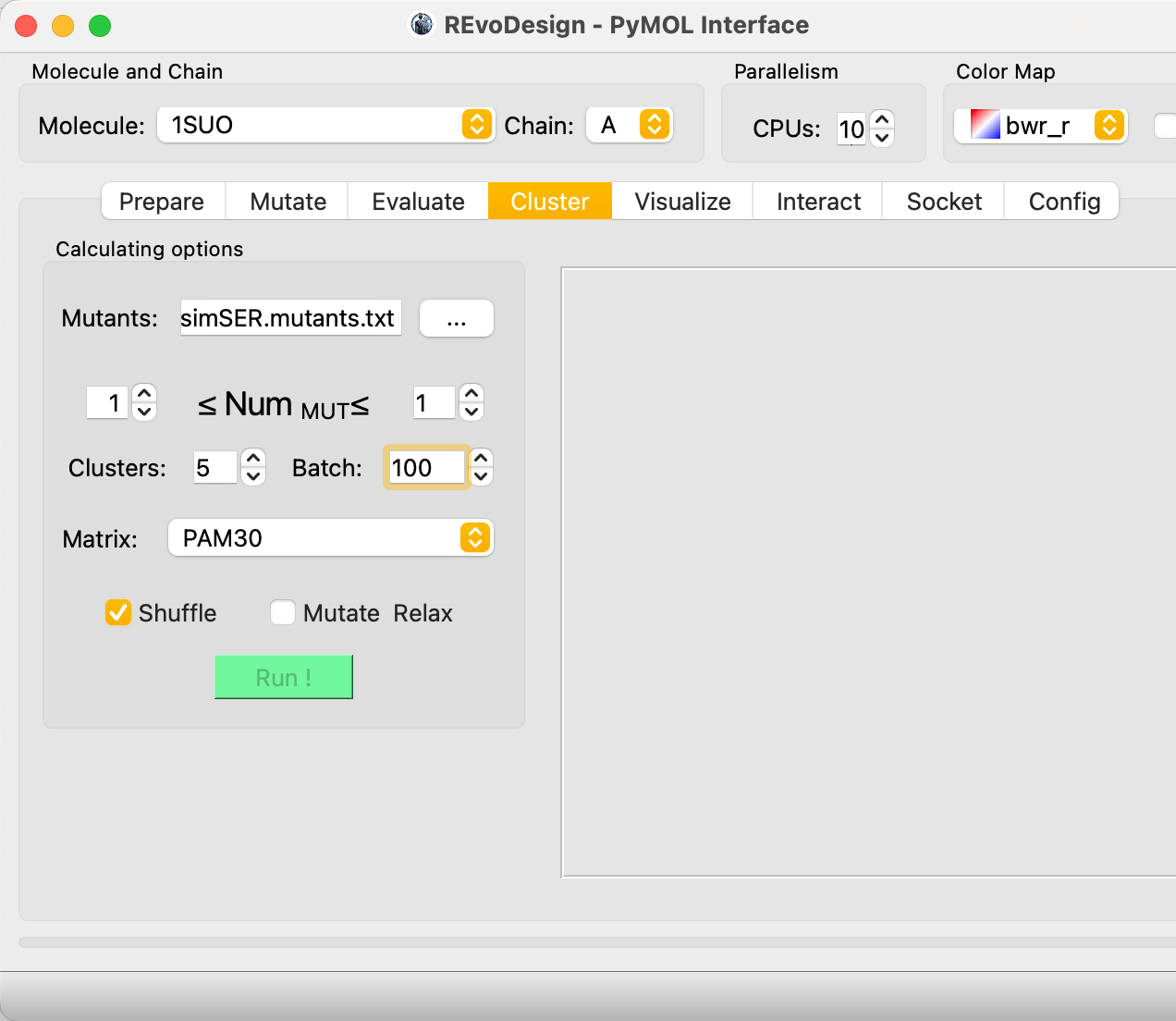
REvoDesign uses sequence-based clustering to group similar mutants and select representatives from each cluster, reducing the library to a size manageable for wet-lab validation.

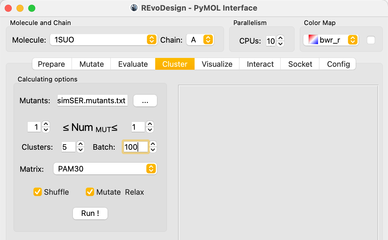
1. Load the accepted mutant list from the Evaluate step.
2. Set the number of mutations per mutant (default: 1).
3. Set the number of clusters (must be less than total mutants).
4. Choose a scoring matrix (default: PAM30).
5. Optionally enable Mutate Relax to score representatives with Rosetta energy evaluation.
6. Click Run.

Sequence clustering parameters

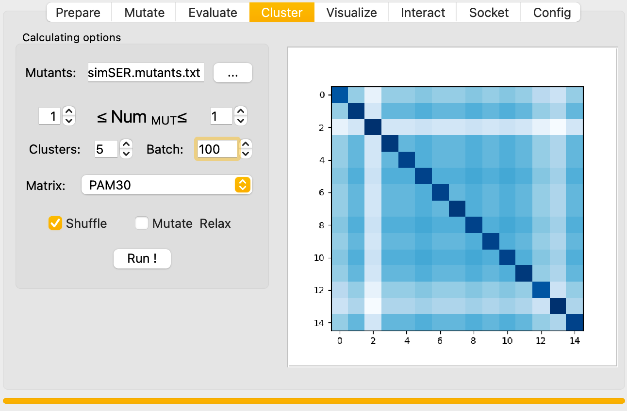
The results panel shows a pairwise sequence similarity matrix (darker = more similar).

Clustering results — matrix shows pairwise sequence similarity

Cluster count

Too few clusters can force unrelated sequences into the same group, masking diversity. Choose a cluster count that balances library size with sequence diversity preservation.

With Rosetta Energy Evaluation

When Mutate Relax is enabled, REvoDesign builds each mutant structure with Rosetta and evaluates its energy. The lowest-energy mutant in each cluster is selected as the representative.

Enabling Rosetta Mutate Relax in clustering

Scoring summary in the log output

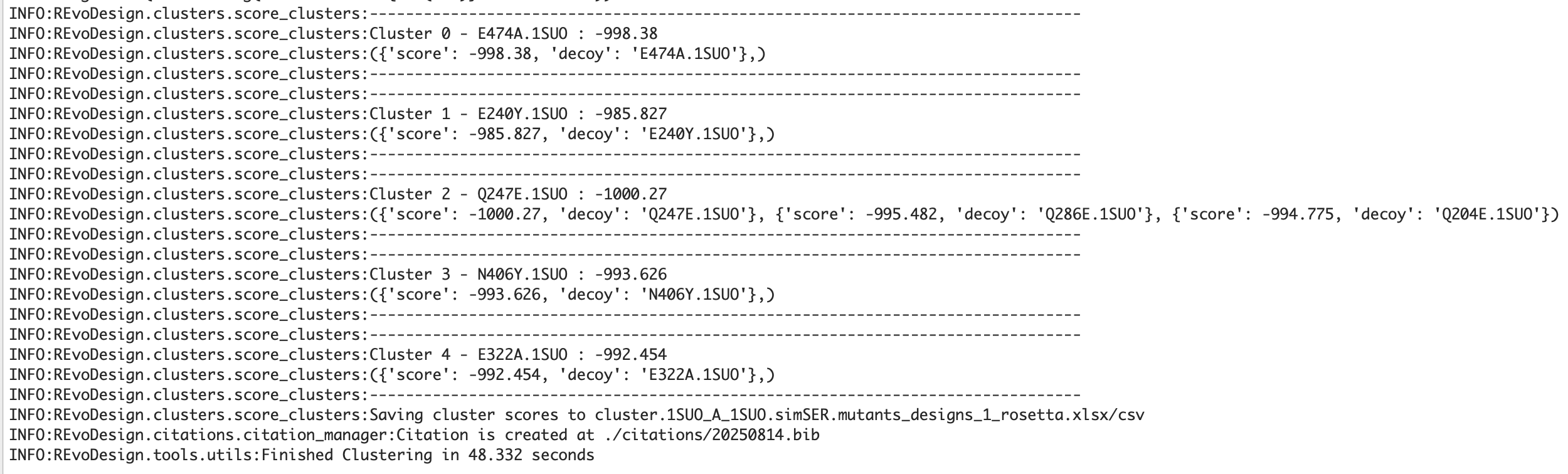
Full scoring results are saved as both Excel and CSV files for downstream analysis.

Mutate Relax assumptions

Mutate Relax operates under three assumptions:

1. The starting structure is already energy-minimized.
2. Point mutations do not affect backbone coordinates.
3. Point mutations do not affect distant sidechain packing.

Under these assumptions, only the mutated site is repacked locally. A well-optimized starting structure is critical for reliable scores.

Step 5: Visualize — Cross-Screening and Data Display

The Visualize tab has two main functions:

Cross-Screening with External Scoring Tools

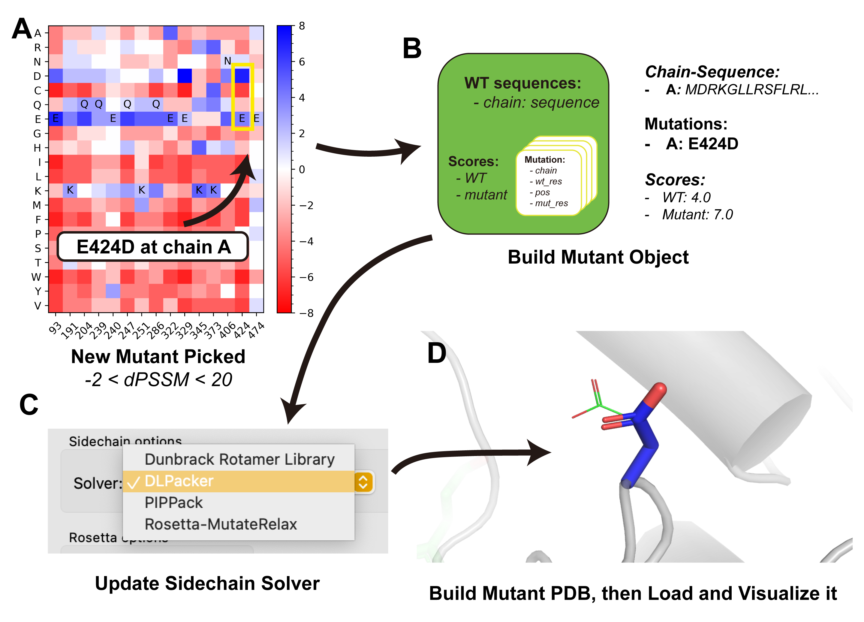
Combine REvoDesign's mutation list with scores from external tools (ddG predictors, stability predictors, etc.) for multi-criteria filtering.

This example uses Pythia-ddG, a structure-based ΔΔG predictor available on BioLib at https://biolib.com/YaoYinYing/pythia-wubianlab/.

Pythia-ddG hosted on BioLib

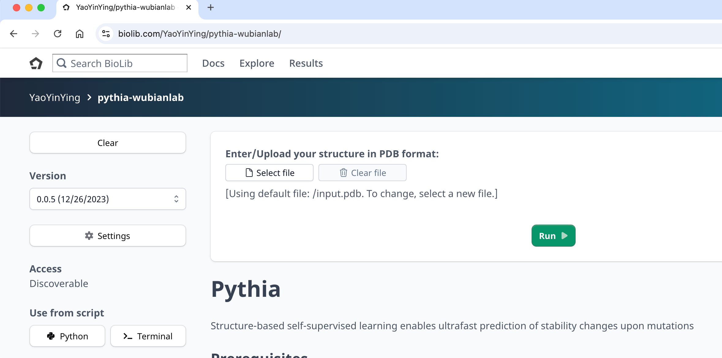
1. Upload the PDB structure to Pythia-ddG and run (takes ~1 minute).
2. Download the CSV results.
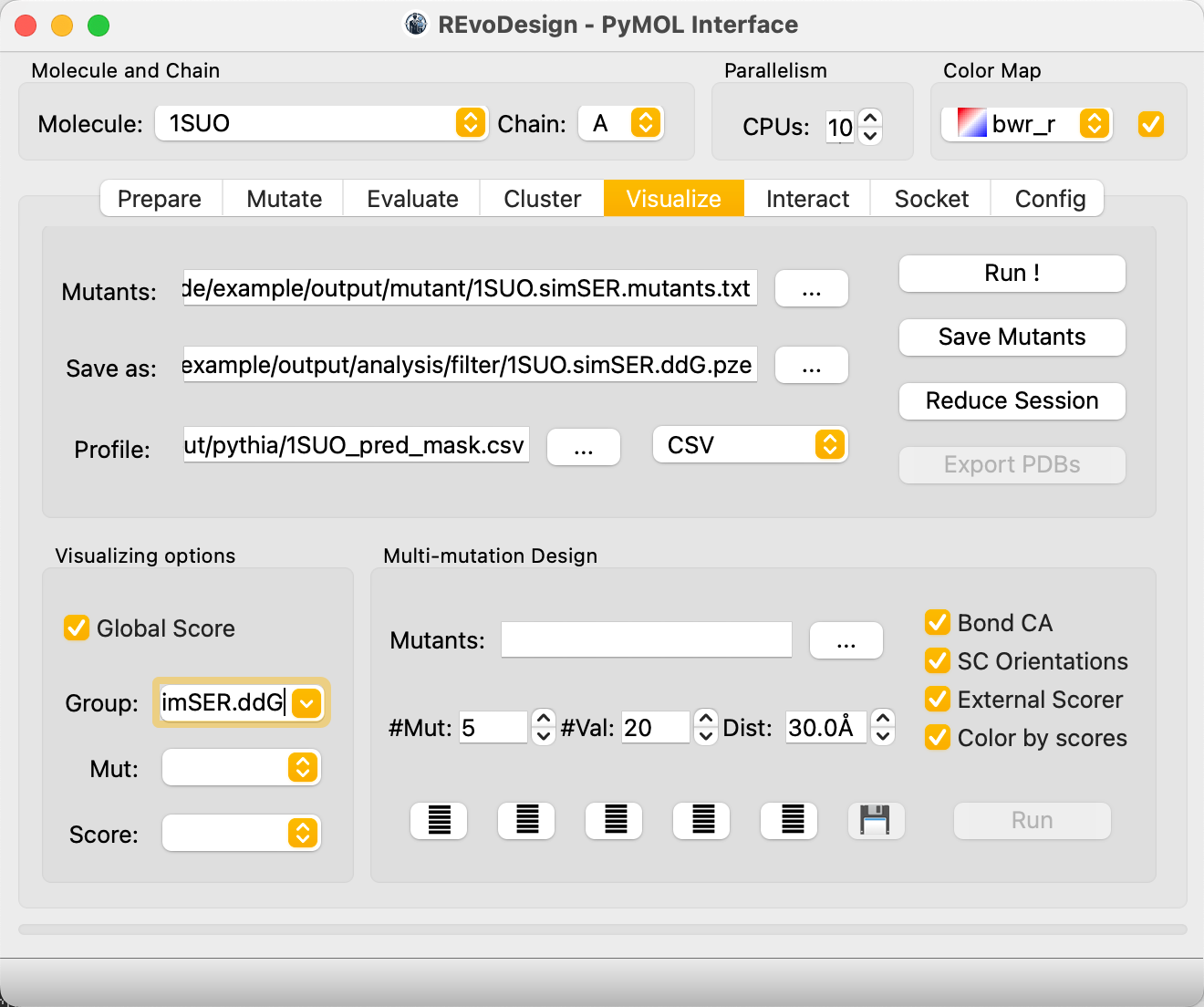
3. In REvoDesign's Visualize tab:
   • Load the mutant list.
   • Set the save path.
   • Select the Pythia-ddG CSV as the profile.
   • Verify Profile type is set to CSV.
   • Check Invert color preset (lower ddG = more stable = better).
   • Check Global scoring to use full-table extremes for coloring.
   • Enter a Group name for MutantTree organization.

Cross-screening configuration with external profile data

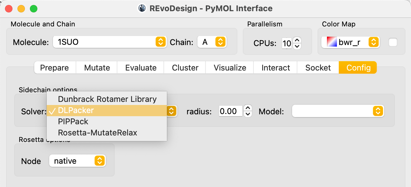
Sidechain solver for cross-screening

When building mutant structures for cross-screening, use a high-accuracy sidechain solver like DLPacker for reliable structural details during visual inspection.

Adjust the sidechain solver for cross-screening accuracy

Pruning the MutantTree

Unwanted mutants can be removed during cross-screening review:

Cross-screening mutant sidechain display

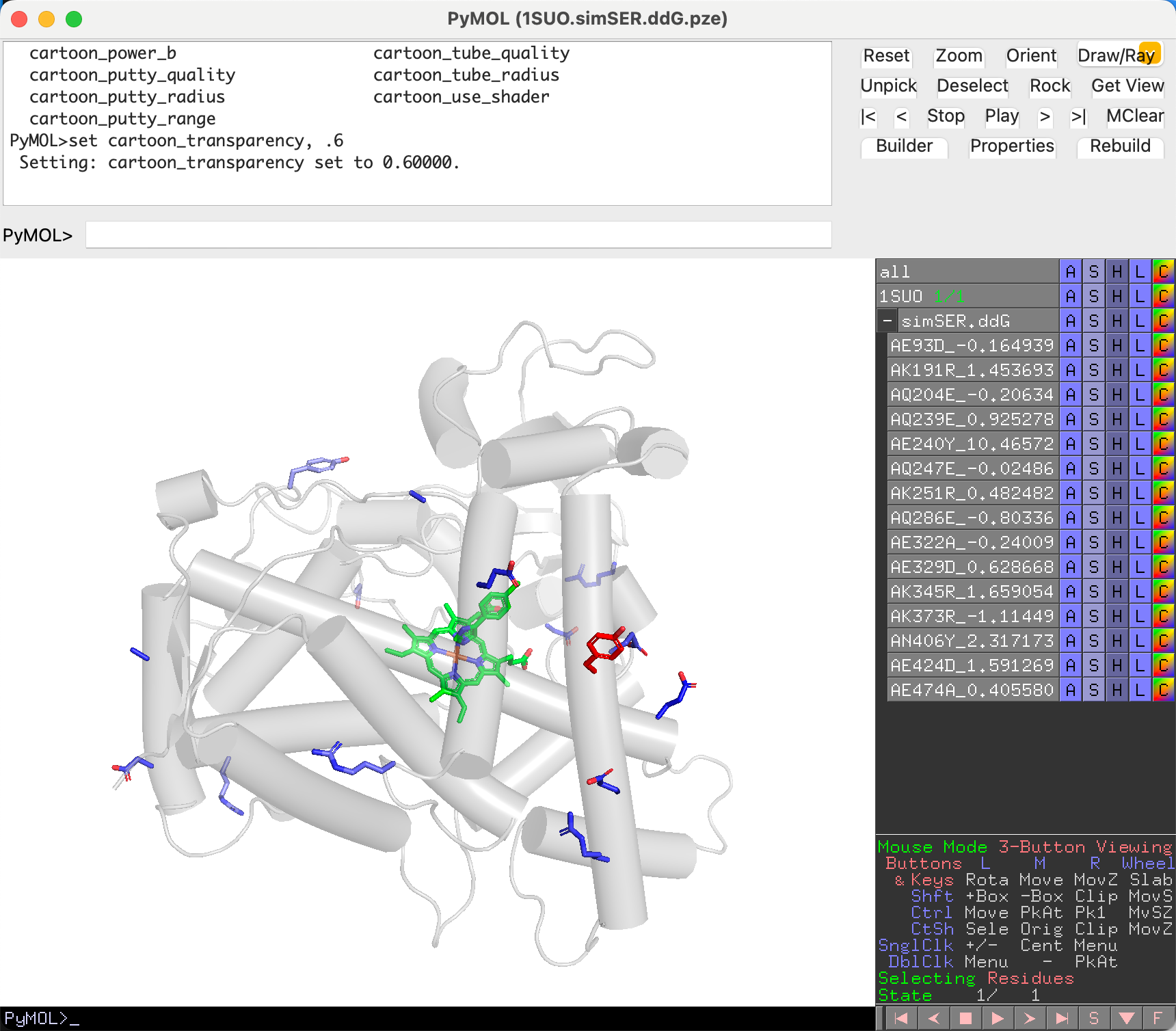
1. Click a mutant in the PyMOL viewer to select it.
2. Click Hide on the right panel to mark it for removal.

Step 1: Click "Hide" on the unwanted mutant

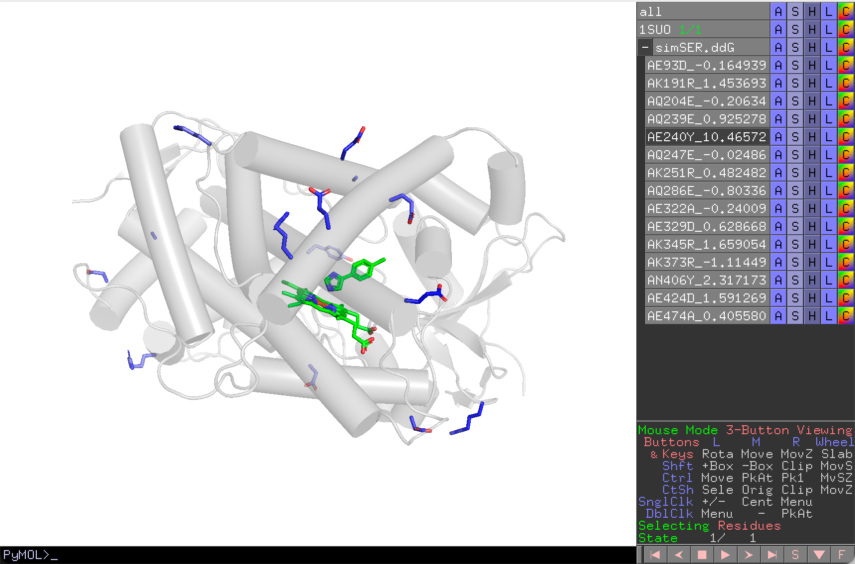
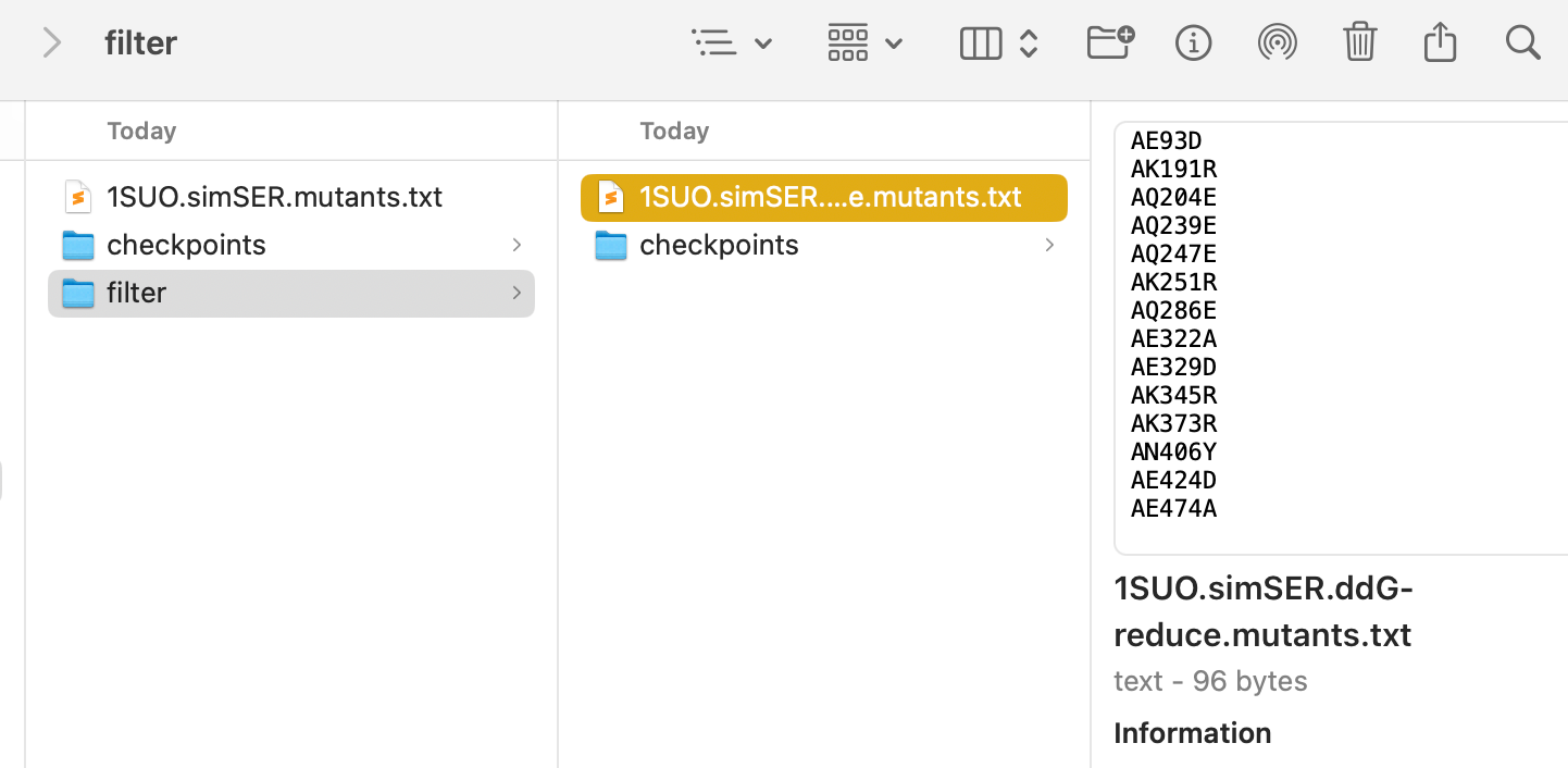
1. Click Reduce Session to delete hidden mutants.

Step 2: Reduce Session to delete, then rename and Save Mutant

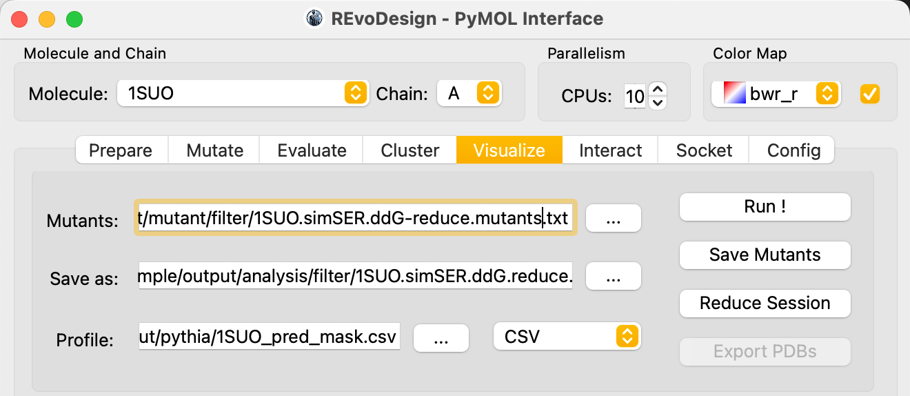
1. Rename the mutant table and click Save Mutant to persist.

Pruned mutant table — unwanted entries removed

PSSM-based coloring of mutation scores on the 3D structure

Displaying Experimental Data on Structure

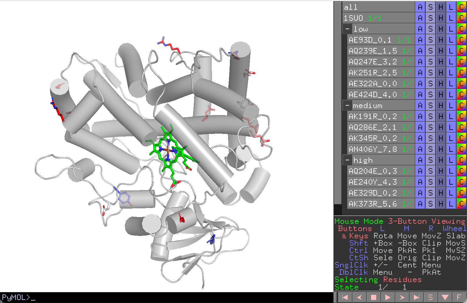
Map your experimental assay results (e.g., enzyme activity, product titer) onto the 3D structure for visual analysis:

1. Prepare a CSV or Excel table:

   mutant	normalized	group
   WT_1	0	control
   wt_2	-0.1	control
   WT	0	control
   AE93D	0.1	low
   AK191R	0.2	medium
   AQ204E	0.3	high

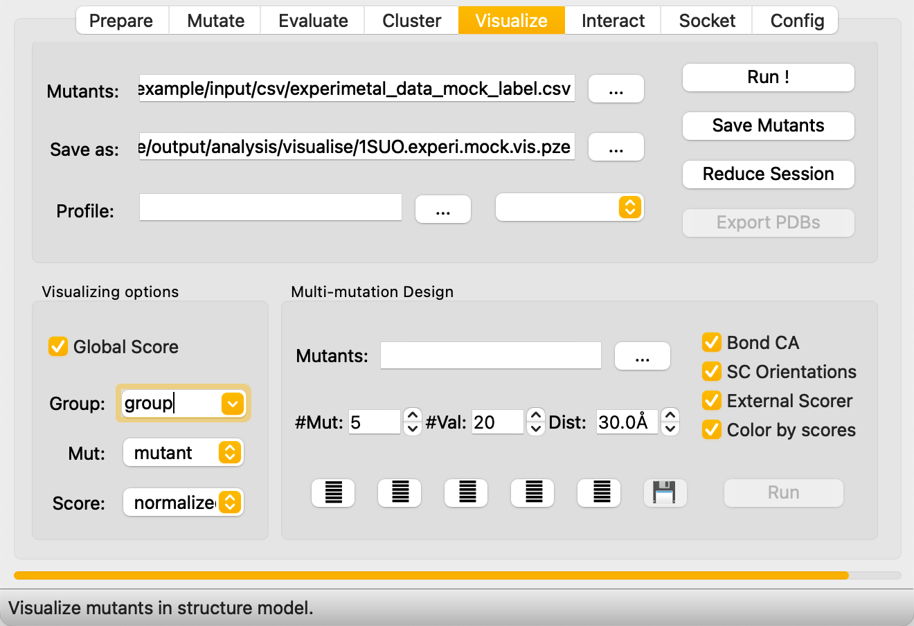
2. In the Visualize tab:

   • Set Mutants to the CSV path.
   • Set Save as to the session save path.
   • Clear the Profile path.
   • Set Profile type to empty.
   • Map column names: Group, Mut, Score to the appropriate CSV column names.

Map CSV columns to Group, Mutant name, and Score

Experimental data mapped onto the 3D structure

WT handling

Rows whose mutant name contains "WT" (case-insensitive) are treated as controls. Their group assignment is ignored and the WT score is set to the average of all control rows.

GREMLIN co-evolution analysis: contact map and residue pair visualization

Step 6: Interact — Co-Evolution Analysis

The Interact tab uses GREMLIN Markov Random Field (MRF) models to identify co-evolved residue pairs, revealing functional coupling between positions that can guide combinatorial mutation design.

Load GREMLIN Data

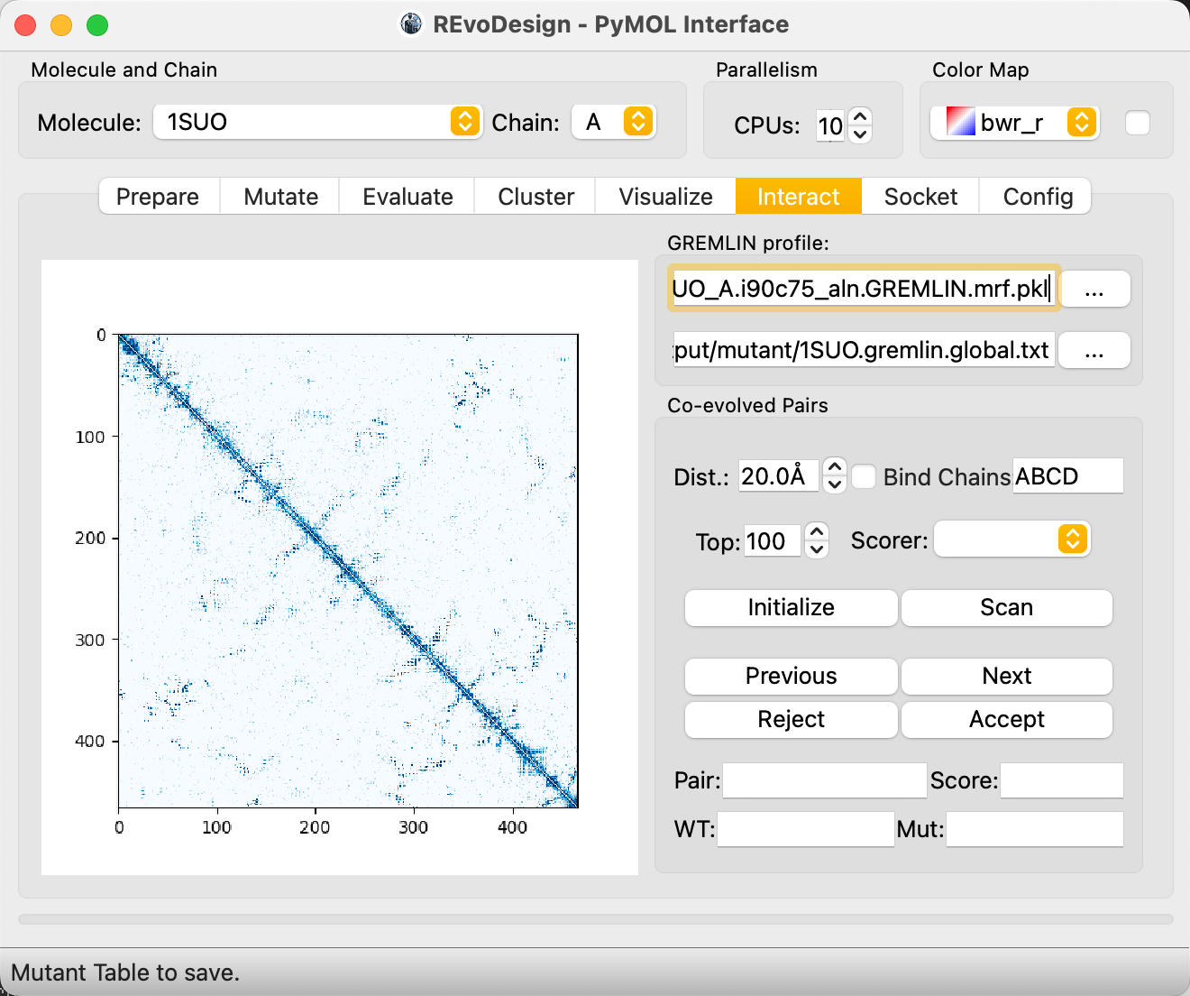
1. In the Interact tab, set the path to the GREMLIN MRF archive (e.g., gremlin_res/1SUO_A.i90c75_aln.GREMLIN.mrf.pkl).
2. Set the mutant design save path.
3. Adjust filters: top N co-evolving pairs, maximum contact distance, homo-oligomer chain binding mode.
4. Optionally enable scoring tools for on-the-fly mutant evaluation.
5. Click Initialize to load the co-evolution contact map.

Co-evolution analysis interface with GREMLIN contact map

Global Co-Evolution Scan

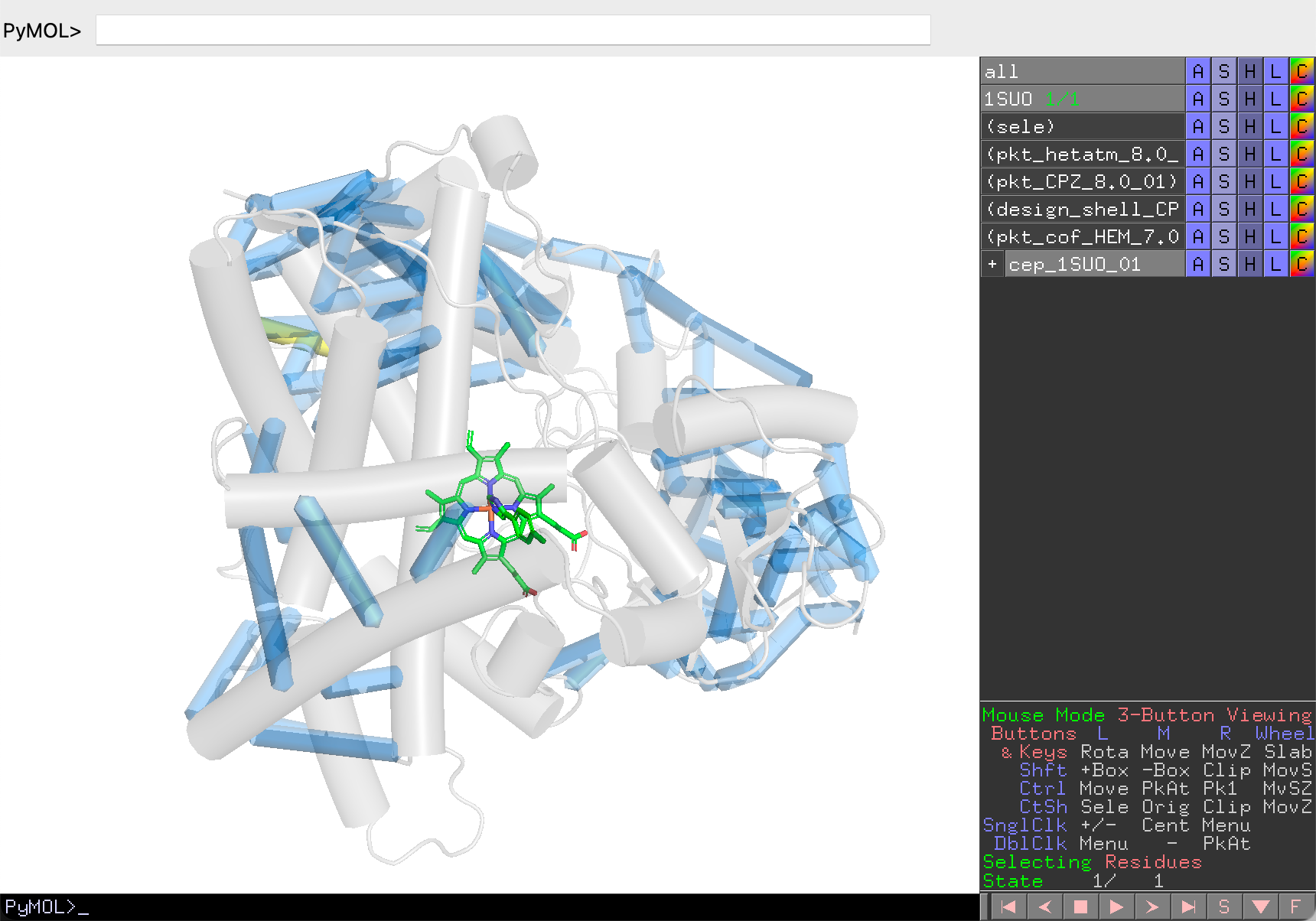
1. Click Scan to analyze the top co-evolving pairs within the distance cutoff.
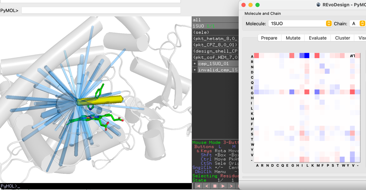
2. Results are displayed as backbone traces: blue cylinders represent pairs, a yellow cylinder highlights the current pair. Cylinder thickness indicates co-evolution signal strength.

Global co-evolution pair scan results

1. Navigate pairs with Previous / Next.
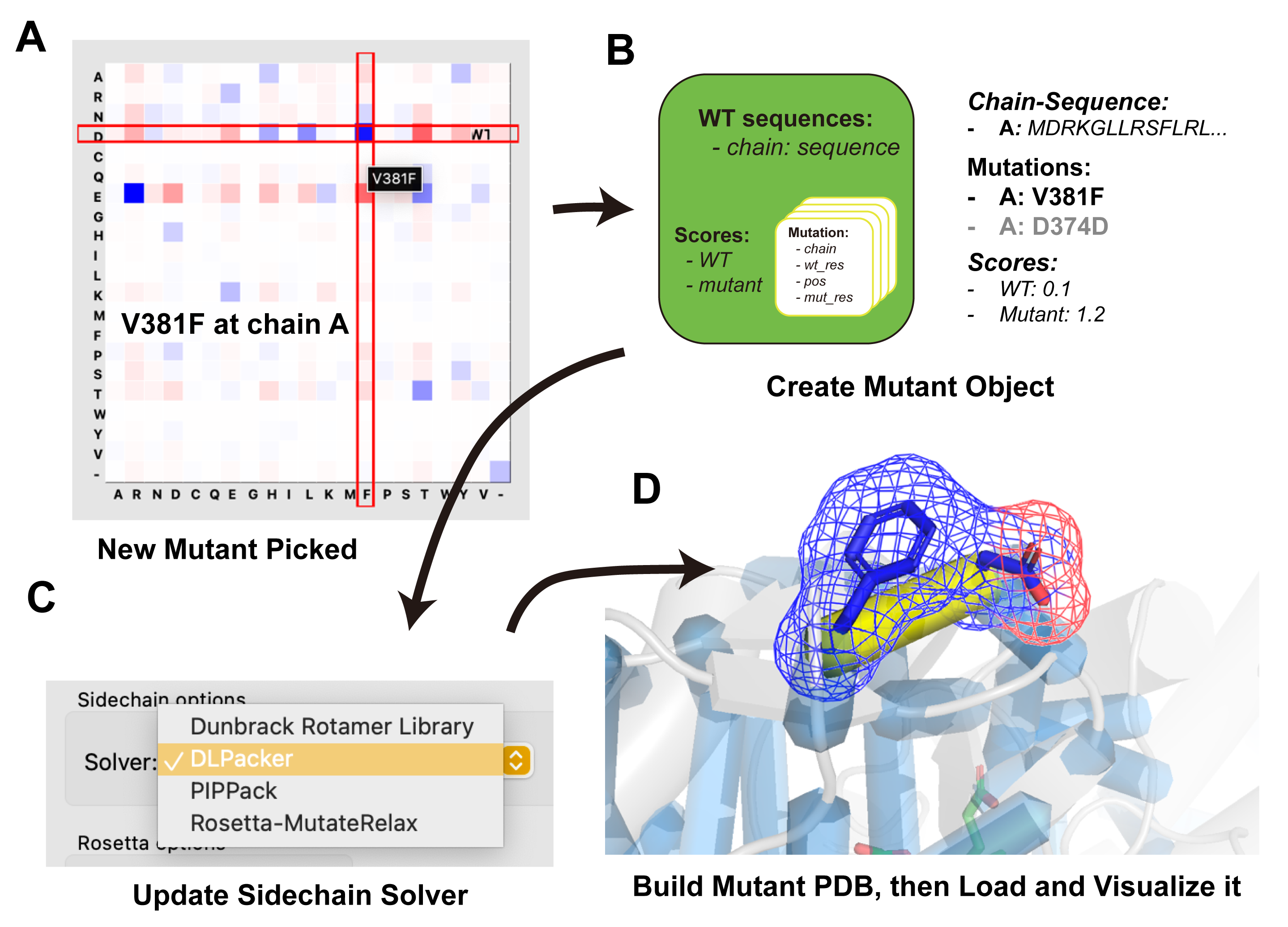
2. For each pair, the MRF matrix shows the 20×20 amino acid combination space. Grid cell color represents the GREMLIN probability for that residue pair.
3. Click any cell to instantly generate the corresponding double mutant. The mutant flows through: build → sidechain modeling → scoring (if enabled) → grouping → display.

Interactive MRF matrix — hover for pair info, click to design a double mutant

Double mutant designed from co-evolution matrix click

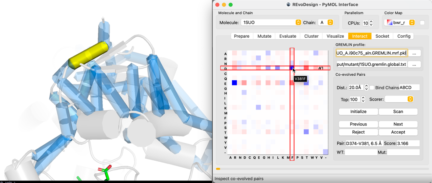
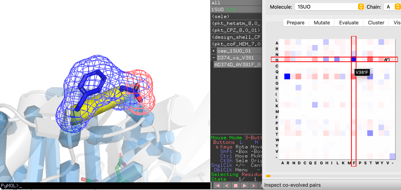
The WT cell marks the wild-type residue combination at the current pair.

Local Co-Evolution Analysis

Local analysis focuses on co-evolution partners of a single residue of interest:

1. In PyMOL, click on a residue to create a sele selection object. (Or use: select sele, 1SUO and resi 298)
2. Ensure the sele selection is enabled (shown/active in PyMOL).
3. Click Scan in the Interact tab.

Local co-evolution analysis — select a residue in PyMOL first

Local co-evolution scan — only pairs involving the selected residue

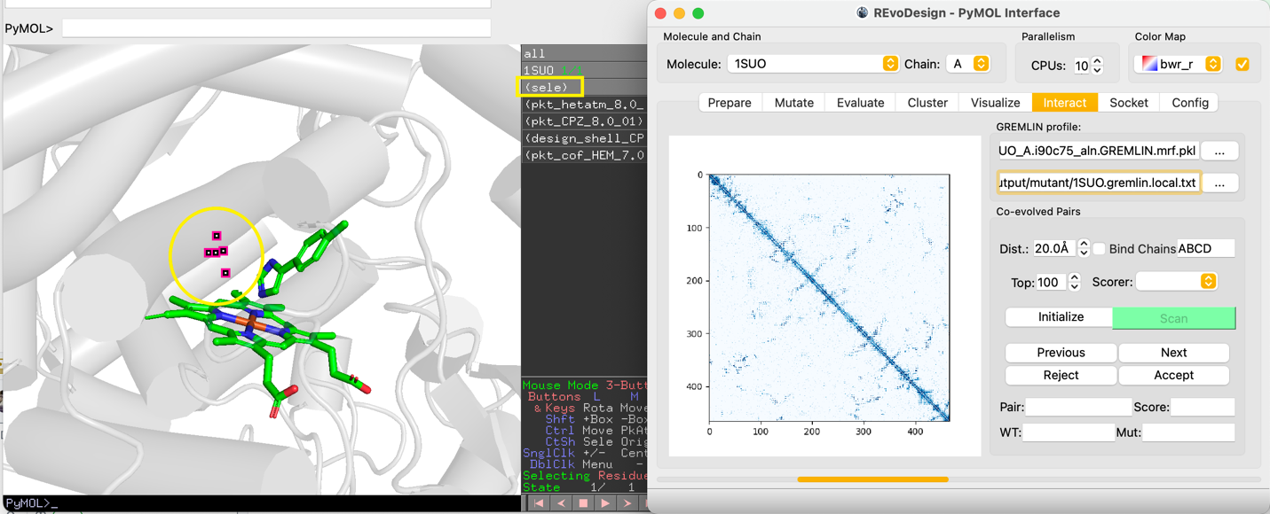
Mutants designed from GREMLIN analysis must be explicitly saved — either click Accept in the Interact tab or switch to the Evaluate tab for structured rational screening.